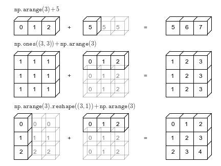
6. Computation on Arrays: Broadcasting
2025. 6. 17. 09:19ㆍPython/Numpy
Introducing Broadcasting
# In[1]
a=np.array([0,1,2])
M=np.ones((3,3))
M+a
# Out[1]
array([[1., 2., 3.],
[1., 2., 3.],
[1., 2., 3.]])- the one-dimensional array
ais stretched(broadcasted), across the second dimension in order to match the shape ofM.
# In[2]
a=np.arange(3)
b=np.arange(3)[:,np.newaxis]
print(a)
print(b)
print(a+b)
# Out[2]
[0 1 2]
[[0]
[1]
[2]]
[[0 1 2]
[1 2 3]
[2 3 4]]aandbboth stretched or broadcasted to match a common shape, and the result is a two-dimensional array.
Rules of Broadcasting
- Rule 1 : If the two arrays differ in their number of dimensions, the shape of the one with fewer dimensions is padded with ones on its leading(left) side.
- Rule 2 : If the shape of the two arrays does not match in any dimension, the array with shape equal to 1 in that dimension is stretched to match the other shape.
- Rule 3 : If in any dimension the sizes disagree and neither is equal to 1, an error is raised.
Broadcasting Example 1
# In[3]
M=np.ones((2,3))
a=np.arange(3)M.shapeis (2,3) , anda.shapeis (3,)- We see by rule 1 that the array
ahas fewer dimensions, so we pad it on the left with ones.
So,M.shaperemains (2,3),a.shapebecomes (1,3) - By rule 2, we see that the first dimension disagrees, so we stretch this dimension to match.
So,M.shaperemains (2,3),a.shapebecomes (2,3)
# In[4]
M+a
# Out[4]
array([[1.,2.,3.],
[1.,2.,3.]])Broadcasting Example 2
# In[5]
a=np.arange(3).reshape((3,1))
b=np.arange(3)a.shapeis (3,1), andb.shapeis (3,)- By rule 1,
a.shaperemains (3,1), andb.shapebecomes (1,3) - By rule 2,
a.shapebecomes (3,3), andb.shapebecomes (3,3)
# In[6]
a+b
# Out[6]
array([[0,1,2],
[1,2,3],
[2,3,4]])Broadcasting Example 3
# In[7]
M=np.ones((3,2))
a=np.arange(3)M.shapeis (3,2), anda.shapeis (3,)- By rule 1,
M.shaperemains (3,2), anda.shapebecomes (1,3) - By rule 2,
M.shaperemains (3,2), anda.shapebecomes (3,3) - By rule3, the final shape do not match, so these two arrays are incompatible.
Broadcasting in Practice
Centering an array
# In[8]
X=np.random.random((10,3))
print(X)
# Out[8]
[[0.79578526 0.06970127 0.80572102]
[0.49596132 0.4203202 0.46907811]
[0.14083824 0.66032281 0.86455548]
[0.06037715 0.83184264 0.54172137]
[0.38316786 0.05267514 0.70413834]
[0.05020395 0.78665839 0.7274787 ]
[0.47849237 0.98020416 0.44380548]
[0.58073628 0.97996138 0.40468001]
[0.25097966 0.39015983 0.79417086]
[0.39169738 0.96715734 0.56671287]]# In[9]
Xmean=X.mean(0) # X.mean('axis')
Xmean# Out[9]
array([0.36282395, 0.61390031, 0.63220622])- We can center the
Xarray by subtracting the mean
# In[10]
X_centered=X-Xmean
X_centered.mean(0)
# Out[10]
array([ 6.66133815e-17, -4.44089210e-17, -6.66133815e-17])Plotting a two-dimensional function
# In[11]
x=np.linspace(0,5,50)
y=np.linspace(0,5,50)[:,np.newaxis]
z=np.sin(x)**10+np.cos(10+y*x)*np.cos(x)
# In[12]
%matplotlib inline
import matplotlib.pyplot as plt
plt.imshow(z,origin='lower',extent=[0,5,0,5],cmap='viridis')
plt.colorbar();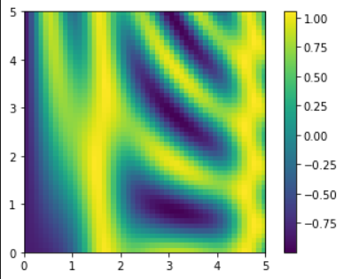
- We can see the result that is a compelling visualization of the two-dimensional function above the image.
References:
1) https://jakevdp.github.io/PythonDataScienceHandbook/02.05-computation-on-arrays-broadcasting.html
'Python > Numpy' 카테고리의 다른 글
| 8. Fancy Indexing (2) | 2025.06.17 |
|---|---|
| 7. Comparisons, Masks, and Boolean Logic (0) | 2025.06.17 |
| 5. Aggregations: Min, Max, and Everything in Between (0) | 2025.06.17 |
| 4. [Ref] About the 'axis' (1) | 2025.06.17 |
| 3. Computation on Numpy Arrays : Universal Functions (0) | 2025.06.17 |